Reproducing Figure 1 of the 2023 SunPy Paper in 2025

import warnings; warnings.simplefilter("ignore")
import logging, sunpy; logging.getLogger('sunpy').setLevel(logging.ERROR)

The SunPy (The SunPy Community et al. 2020) is a community-developed, free, and open source Python package for solar data analysis (Barnes et al. 2023; Mumford et al. 2020; The SunPy Community et al. 2015).

In this post, I will reproduce Figure 1 (see below) of the 2023 SunPy paper (Barnes et al. 2023) using the SunPy ecosystem. This is because one of the most important affiliated packages, pfsspy (Stansby et al. 2020), has been no longer developed since August 2023. The pfsspy package has been forked to sunkit-magex. Also, there are subtle differences in the aiapy package between 2023 and 2025. Therefore, I will basically follow the steps in this code provided by the authors of the 2023 SunPy paper, except that I will use the sunkit-magex package instead of the pfsspy package.

Version Information

import sys
print("Python version:", sys.version)

import numpy as np
print("NumPy version:", np.__version__)
import matplotlib
print("Matplotlib version:", matplotlib.__version__)
import astropy
print("Astropy version:", astropy.__version__)
import sunpy
print("SunPy version:", sunpy.__version__)
import aiapy
print("aiapy version:", aiapy.__version__)
import sunpy_soar
print("sunpy-soar version:", sunpy_soar.__version__)
import sunkit_magex
print("sunkit-magex version:", sunkit_magex.__version__)

Python version: 3.12.11 | packaged by conda-forge | (main, Jun  4 2025, 14:29:09) [MSC v.1943 64 bit (AMD64)]
NumPy version: 2.2.6
Matplotlib version: 3.10.5
Astropy version: 7.1.0
SunPy version: 7.0.1
aiapy version: 0.10.1
sunpy-soar version: 1.11.1
sunkit-magex version: 1.1.0

Download HMI Synoptic Magnetogram for CR 2255

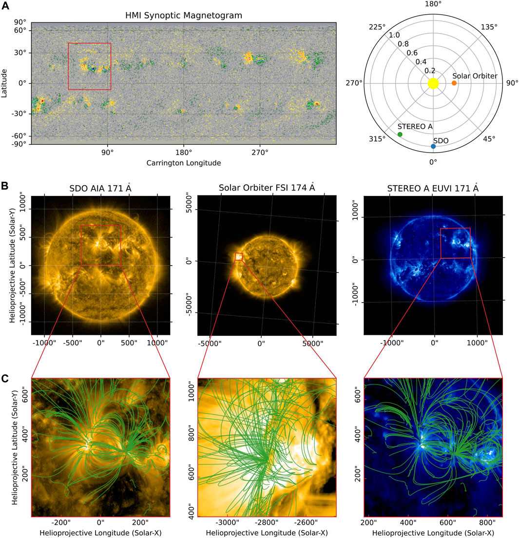
The SunPy paper (2023) said that the left panel of Figure1A shows the SDO/HMI synoptic magnetogram for Carrington rotation (CR) 2255 which began on 2022-03-08.

Let’s start by checking that CR 2255 actually began on 2022-03-08.

from sunpy.coordinates.sun import carrington_rotation_time

carrington_rotation_time(2255)

<Time object: scale='utc' format='iso' value=2022-03-07 11:59:56.657>

CR 2255 actually began on 2022-03-07 12:00 UTC, which also can be found in this page.

We can download the HMI polar-filled full-CR synoptic magnetogram hmi.synoptic_mr_polfil_720s (Sun 2018) for CR 2255 from JSOC using sunpy.net.Fido.

from sunpy.net import Fido, attrs as a

# Please replace the following email with your own email address registered with the JSOC.
jsoc_email = ''

q = Fido.search(
    a.Time('2022-03-07T12:00', '2022-03-07T12:00'),
    a.jsoc.Series('hmi.synoptic_mr_polfil_720s'),
    a.jsoc.PrimeKey('CAR_ROT', 2255),
    a.jsoc.Notify(jsoc_email)
)

Results from 1 Provider:

1 Results from the JSOCClient:

JSOCResponse length=1

TELESCOP	INSTRUME	WAVELNTH	CAR_ROT
str7	str9	float64	int64
SDO/HMI	HMI_SIDE1	6173.0	2255

f = Fido.fetch(q, path='./data', overwrite=True)

print(f)

['data\\hmi.synoptic_mr_polfil_720s.2255.Mr_polfil.fits']

We can load the fits file using sunpy.map.Map.

from sunpy.map import Map

m_hmi = Map(f)

m_hmi.peek()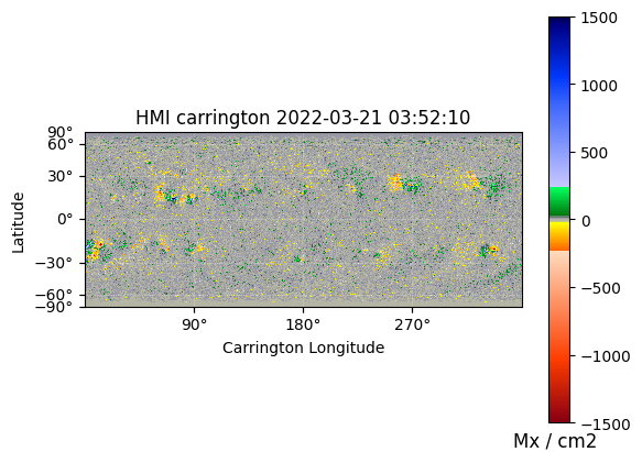

This is the same HMI synoptic magnetogram as shown in the left panel of Figure 1A in the SunPy paper (2023).

Select Location of AR

We identify the center of the active region (AR) of interest visually from the HMI synoptic magnetogram.

import astropy.units as u
from astropy.coordinates import SkyCoord

m_hmi.coordinate_frame

<HeliographicCarrington Frame (obstime=2022-03-21T03:51:33.000, rsun=695700.0 km, observer=<HeliographicStonyhurst Coordinate (obstime=2022-03-21T03:51:33.000, rsun=695700.0 km): (lon, lat, radius) in (deg, deg, m)
    (0., -7.02110576, 1.48994814e+11)>)>

ar_center = SkyCoord(lon=65*u.deg, lat=15*u.deg, frame=m_hmi.coordinate_frame)

We can plot this coordinate on the HMI map.

import matplotlib.pyplot as plt

fig = plt.figure(figsize=(15, 5))
ax = fig.add_subplot(111, projection=m_hmi)
m_hmi.plot(axes=ax)
ax.plot_coord(ar_center, marker='X', color='k', markersize=10);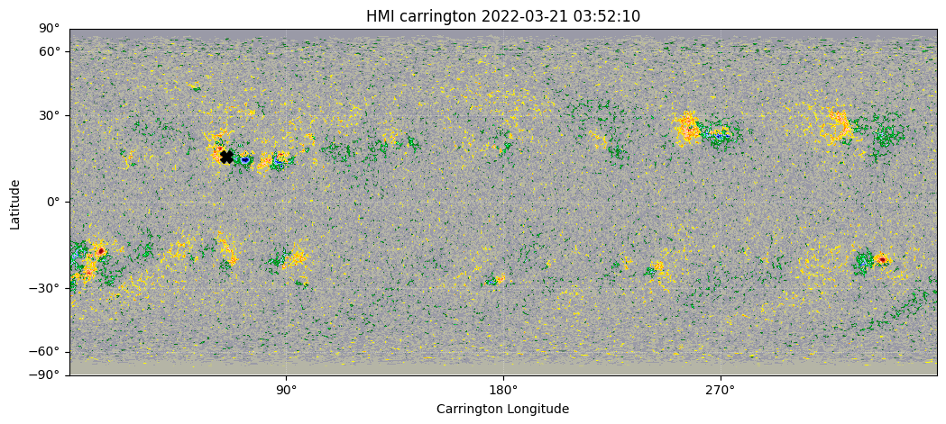

The default obstime of the carrington map is halfway through the carrington rotation.

m_hmi.coordinate_frame.obstime

<Time object: scale='utc' format='isot' value=2022-03-21T03:51:33.000>

car_start = carrington_rotation_time(2255)
car_end = carrington_rotation_time(2256)
print('CR 2255 start   ', car_start)
print('CR 2255 end     ', car_end)
car_halfway = car_start + (car_end - car_start) / 2
print('CR 2255 halfway ', car_halfway)

CR 2255 start    2022-03-07 11:59:56.657
CR 2255 end      2022-04-03 19:19:29.900
CR 2255 halfway  2022-03-21 03:39:43.279

Since a synoptic map is comprised of observations from many different times, we look up the obstime associated with our selected longitude and use this to correct our original AR coordinate

ar_date = carrington_rotation_time(2255, ar_center.lon)
ar_date

<Time object: scale='utc' format='iso' value=2022-03-29 21:04:15.174>

change_obstime = lambda x,y: SkyCoord(x.replicate(observer=x.observer.replicate(obstime=y), obstime=y))

ar_center_corrected = change_obstime(ar_center, ar_date)
ar_center_corrected

<SkyCoord (HeliographicCarrington: obstime=2022-03-29 21:04:15.174, rsun=695700.0 km, observer=<HeliographicStonyhurst Coordinate (obstime=2022-03-29 21:04:15.174, rsun=695700.0 km): (lon, lat, radius) in (deg, deg, m)
    (0., -7.02110576, 1.48994814e+11)>): (lon, lat) in deg
    (65., 15.)>

Download EUV data for AR

We will download the EUV data from SDO/AIA, STEREO-A/SECCHI/EUVI, and Solar Orbiter/EUI/FSI.

First, we define the time range of interest.

tr = a.Time(ar_date-2*u.min, ar_date+2*u.min)
tr

<sunpy.net.attrs.Time(2022-03-29 21:02:15.174, 2022-03-29 21:06:15.174)>

We construct a search query for 171 Å EUV data from SDO/AIA and STEREO-A/SECCHI/EUVI. This will search the Virtual Solar Observatory (VSO).

aia_or_euvi = ((a.Instrument('AIA') | a.Instrument('EUVI'))
                & a.Wavelength(171*u.angstrom)
                & a.Sample(5*u.min))

We construct a search query for 174 Å EUV data from Solar Orbiter/EUI/FSI. This will search the Solar Oriter Archive (SOAR) using the sunpy-soar package.

eui = a.Level(2) & a.soar.Product('EUI-FSI174-IMAGE')

q = Fido.search(tr, aia_or_euvi | eui)

Results from 3 Providers:

1 Results from the VSOClient:

VSOQueryResponseTable length=1

Start Time	End Time	Source	Instrument	Wavelength	Provider	Physobs	Wavetype	Extent Width	Extent Length	Extent Type	Size
				Angstrom							Mibyte
Time	Time	str3	str3	float64[2]	str4	str9	str6	str4	str4	str8	float64
2022-03-29 21:02:21.000	2022-03-29 21:02:22.000	SDO	AIA	171.0 .. 171.0	JSOC	intensity	NARROW	4096	4096	FULLDISK	64.64844

1 Results from the VSOClient:

VSOQueryResponseTable length=1

Start Time	End Time	Source	Instrument	Wavelength	Provider	Physobs	Wavetype	Extent Type	Size
				Angstrom					Mibyte
Time	Time	str8	str6	float64[2]	str3	str9	str6	str8	float64
2022-03-29 21:03:00.000	2022-03-29 21:03:02.000	STEREO_A	SECCHI	171.0 .. 175.0	SSC	intensity	NARROW	FULLDISK	-0.00098

1 Results from the SOARClient:

QueryResponseTable length=1

Instrument	Data product	Level	Start time	End time	Data item ID	Filename	Filesize	SOOP Name	Detector	Wavelength
							Mbyte
str3	str16	str2	str23	str23	str43	str52	float64	str31	str3	float64
EUI	eui-fsi174-image	L2	2022-03-29 21:04:45.298	2022-03-29 21:04:55.298	solo_L2_eui-fsi174-image_20220329T210445298	solo_L2_eui-fsi174-image_20220329T210445298_V02.fits	5.593	L_FULL_HRES_HCAD_Eruption-Watch	FSI	174.0

Note that Fido returns three results (one for each instrument) and that two out of the three of these are from the VSO and one is from the SOAR.

files = Fido.fetch(q, path='./data', overwrite=True)

print(sorted(files))

['data\\20220329_210300_n5euA.fts', 'data\\aia.lev1.171A_2022_03_29T21_02_21.35Z.image_lev1.fits', 'data\\solo_L2_eui-fsi174-image_20220329T210445298_V02.fits']

m_secchi, m_aia, m_eui = Map(sorted(files))

Using the metadata provided in each file, we can plot the relative locations of the three spacecraft.

fig = plt.figure()
ax = fig.add_subplot(111, projection='polar')
# Plot the Sun
ax.plot(0, 0, marker='o', markersize=20, label='Sun', color='yellow')
# Plot the spacecraft locations
for m in [m_aia, m_eui, m_secchi]:
    sat = m.observatory
    coord = m.observer_coordinate
    ax.plot(coord.lon.to('rad'), coord.radius.to(u.AU), 'o', label=sat)
ax.set_theta_zero_location('S')
ax.legend();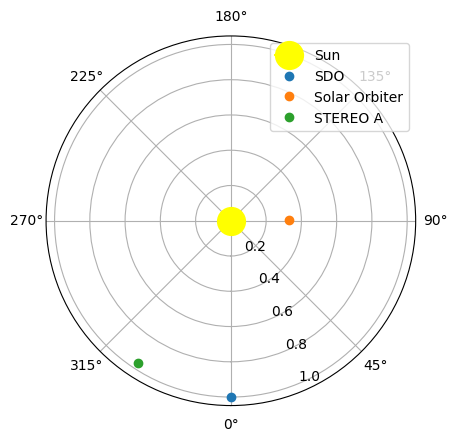

Process EUV Data for AR

We prepare the SDO/AIA data from level 1 to level 1.5 using aiapy package by (1) correcting the pointing keywords and (2) also correcting the instrument degradation.

from aiapy.calibrate import update_pointing, correct_degradation
from aiapy.calibrate.util import get_pointing_table, get_correction_table

pointing_table = get_pointing_table('JSOC', time_range=(m_aia.date-12*u.h, m_aia.date+12*u.h))

pointing_table

QTable length=8

ORIGIN	TELESCOP	DATE	T_START	T_STOP	T_HKVALS	VERSION	SC_Y_INRT_BIAS	SC_Z_INRT_BIAS	H_CAM1_IMSCALE	H_CAM1_X0	H_CAM1_Y0	H_CAM1_INSTROT	H_CAM2_IMSCALE	H_CAM2_X0	H_CAM2_Y0	H_CAM2_INSTROT	A_094_IMSCALE	A_094_X0	A_094_Y0	A_094_INSTROT	A_131_IMSCALE	A_131_X0	A_131_Y0	A_131_INSTROT	A_171_IMSCALE	A_171_X0	A_171_Y0	A_171_INSTROT	A_193_IMSCALE	A_193_X0	A_193_Y0	A_193_INSTROT	A_211_IMSCALE	A_211_X0	A_211_Y0	A_211_INSTROT	A_304_IMSCALE	A_304_X0	A_304_Y0	A_304_INSTROT	A_335_IMSCALE	A_335_X0	A_335_Y0	A_335_INSTROT	A_1600_IMSCALE	A_1600_X0	A_1600_Y0	A_1600_INSTROT	A_1700_IMSCALE	A_1700_X0	A_1700_Y0	A_1700_INSTROT	A_4500_IMSCALE	A_4500_X0	A_4500_Y0	A_4500_INSTROT	HMI_FSW_AL1_POSITION	HAL1POS	HMI_FSW_AL2_POSITION	HAL2POS	HMI_AL1_STATUS	HAL1STAT	HMI_AL2_STATUS	HAL2STAT	HMI_ISS_ERRGAINY	HIERRGNY	HMI_ISS_ERRGAINZ	HIERRGNZ	HMI_ISS_ERROFFY	HIERROFY	HMI_ISS_ERROFFZ	HIERROFZ	HMI_ISS_PZTOFFA	HIPZTOFA	HMI_ISS_PZTOFFB	HIPZTOFB	HMI_ISS_PZTOFFC	HIPZTOFC	HMI_ISS_PKT_YCOEF_A	HIYCOEFA	HMI_ISS_PKT_YCOEF_B	HIYCOEFB	HMI_ISS_PKT_YCOEF_C	HIYCOEFC	HMI_ISS_PKT_ZCOEF_A	HIZCOEFA	HMI_ISS_PKT_ZCOEF_B	HIZCOEFB	HMI_ISS_PKT_ZCOEF_C	HIZCOEFC	AIA_IS1_ERRGAINY	A1ERRGNY	AIA_IS1_ERRGAINZ	A1ERRGNZ	AIA_IS1_ERROFFY	A1ERROFY	AIA_IS1_ERROFFZ	A1ERROFZ	AIA_IS1_PZTGAINA	A1PZTGNA	AIA_IS1_PZTGAINB	A1PZTGNB	AIA_IS1_PZTGAINC	A1PZTGNC	AIA_IS1_PZTOFFA	A1PZTOFA	AIA_IS1_PZTOFFB	A1PZTOFB	AIA_IS1_PZTOFFC	A1PZTOFC	AIA_GT1_PKT_YCOEF_A	AGT1_YCA	AIA_GT1_PKT_YCOEF_B	AGT1_YCB	AIA_GT1_PKT_YCOEF_C	AGT1_YCC	AIA_GT1_PKT_ZCOEF_A	AGT1_ZCA	AIA_GT1_PKT_ZCOEF_B	AGT1_ZCB	AIA_GT1_PKT_ZCOEF_C	AGT1_ZCC	AIA_IS2_ERRGAINY	A2ERRGNY	AIA_IS2_ERRGAINZ	A2ERRGNZ	AIA_IS2_ERROFFY	A2ERROFY	AIA_IS2_ERROFFZ	A2ERROFZ	AIA_IS2_PZTGAINA	A2PZTGNA	AIA_IS2_PZTGAINB	A2PZTGNB	AIA_IS2_PZTGAINC	A2PZTGNC	AIA_IS2_PZTOFFA	A2PZTOFA	AIA_IS2_PZTOFFB	A2PZTOFB	AIA_IS2_PZTOFFC	A2PZTOFC	AIA_GT2_PKT_YCOEF_A	AGT2_YCA	AIA_GT2_PKT_YCOEF_B	AGT2_YCB	AIA_GT2_PKT_YCOEF_C	AGT2_YCC	AIA_GT2_PKT_ZCOEF_A	AGT2_ZCA	AIA_GT2_PKT_ZCOEF_B	AGT2_ZCB	AIA_GT2_PKT_ZCOEF_C	AGT2_ZCC	AIA_IS3_ERRGAINY	A3ERRGNY	AIA_IS3_ERRGAINZ	A3ERRGNZ	AIA_IS3_ERROFFY	A3ERROFY	AIA_IS3_ERROFFZ	A3ERROFZ	AIA_IS3_PZTGAINA	A3PZTGNA	AIA_IS3_PZTGAINB	A3PZTGNB	AIA_IS3_PZTGAINC	A3PZTGNC	AIA_IS3_PZTOFFA	A3PZTOFA	AIA_IS3_PZTOFFB	A3PZTOFB	AIA_IS3_PZTOFFC	A3PZTOFC	AIA_GT3_PKT_YCOEF_A	AGT3_YCA	AIA_GT3_PKT_YCOEF_B	AGT3_YCB	AIA_GT3_PKT_YCOEF_C	AGT3_YCC	AIA_GT3_PKT_ZCOEF_A	AGT3_ZCA	AIA_GT3_PKT_ZCOEF_B	AGT3_ZCB	AIA_GT3_PKT_ZCOEF_C	AGT3_ZCC	AIA_IS4_ERRGAINY	A4ERRGNY	AIA_IS4_ERRGAINZ	A4ERRGNZ	AIA_IS4_ERROFFY	A4ERROFY	AIA_IS4_ERROFFZ	A4ERROFZ	AIA_IS4_PZTGAINA	A4PZTGNA	AIA_IS4_PZTGAINB	A4PZTGNB	AIA_IS4_PZTGAINC	A4PZTGNC	AIA_IS4_PZTOFFA	A4PZTOFA	AIA_IS4_PZTOFFB	A4PZTOFB	AIA_IS4_PZTOFFC	A4PZTOFC	AIA_GT4_PKT_YCOEF_A	AGT4_YCA	AIA_GT4_PKT_YCOEF_B	AGT4_YCB	AIA_GT4_PKT_YCOEF_C	AGT4_YCC	AIA_GT4_PKT_ZCOEF_A	AGT4_ZCA	AIA_GT4_PKT_ZCOEF_B	AGT4_ZCB	AIA_GT4_PKT_ZCOEF_C	AGT4_ZCC
									arcsec / pix	pix	pix	deg	arcsec / pix	pix	pix	deg	arcsec / pix	pix	pix	deg	arcsec / pix	pix	pix	deg	arcsec / pix	pix	pix	deg	arcsec / pix	pix	pix	deg	arcsec / pix	pix	pix	deg	arcsec / pix	pix	pix	deg	arcsec / pix	pix	pix	deg	arcsec / pix	pix	pix	deg	arcsec / pix	pix	pix	deg	arcsec / pix	pix	pix	deg
str12	str3	str20	Time	Time	str20	int64	float64	float64	float64	float64	float64	float64	float64	float64	float64	float64	float64	float64	float64	float64	float64	float64	float64	float64	float64	float64	float64	float64	float64	float64	float64	float64	float64	float64	float64	float64	float64	float64	float64	float64	float64	float64	float64	float64	float64	float64	float64	float64	float64	float64	float64	float64	float64	float64	float64	float64	float64	float64	float64	float64	float64	float64	float64	float64	float64	float64	float64	float64	float64	float64	float64	float64	float64	float64	float64	float64	float64	float64	float64	float64	float64	float64	float64	float64	float64	float64	float64	float64	float64	float64	float64	float64	float64	float64	float64	float64	float64	float64	float64	float64	float64	float64	float64	float64	float64	float64	float64	float64	float64	float64	float64	float64	float64	float64	float64	float64	float64	float64	float64	float64	float64	float64	float64	float64	float64	float64	float64	float64	float64	float64	float64	float64	float64	float64	float64	float64	float64	float64	float64	float64	float64	float64	float64	float64	float64	float64	float64	float64	float64	float64	float64	float64	float64	float64	float64	float64	float64	float64	float64	float64	float64	float64	float64	float64	float64	float64	float64	float64	float64	float64	float64	float64	float64	float64	float64	float64	float64	float64	float64	float64	float64	float64	float64	float64	float64	float64	float64	float64	float64	float64	float64	float64	float64	float64	float64	float64	float64	float64	float64	float64	float64	float64	float64	float64	float64	float64	float64	float64	float64	float64	float64	float64	float64	float64	float64	float64	float64	float64
SDO/JSOC-SDP	SDO	2022-03-30T16:51:58Z	2022-03-29T12:00:00.000	2022-03-29T18:00:00.000	2022-03-27T00:00:00Z	1	-4.983	9.323	0.50489	2033.790039	2051.580078	180.013504	0.50486	2039.630005	2048.47998	179.929794	0.600109	2069.821533	2009.129517	-0.13761	0.600698	2041.704346	2041.861694	-0.138795	0.599489	2054.610596	2047.310181	0.019327	0.600714	2040.759888	2041.918091	0.057789	0.600758	2036.590942	2040.456055	0.056433	0.600165	2067.379883	2006.143433	-0.131639	0.600737	2040.537598	2040.539795	-0.142443	0.609373	2051.854492	2046.561401	0.019792	0.612898	2053.222168	2044.922974	0.020525	0.599945	2051.936768	2048.193359	0.020638	76.0	76.0	44.0	44.0	81.0	81.0	81.0	81.0	-43.0	-43.0	-44.0	-44.0	-37.0	-37.0	66.0	66.0	-16.0	-16.0	-16.0	-16.0	-13.0	-13.0	-20920.0	-20920.0	-10460.0	-10460.0	-10460.0	-10460.0	0.0	0.0	-15098.0	-15098.0	-15098.0	-15098.0	-85.0	-85.0	-85.0	-85.0	-17.0	-17.0	53.0	53.0	-20.0	-20.0	-19.0	-19.0	-19.0	-19.0	-15.0	-15.0	-17.0	-17.0	32.0	32.0	2048.0	2048.0	13900.0	13900.0	0.0	0.0	2048.0	2048.0	13900.0	13900.0	0.0	0.0	-85.0	-85.0	-85.0	-85.0	1.0	1.0	38.0	38.0	-18.0	-18.0	-30.0	-30.0	-30.0	-30.0	11.0	11.0	5.0	5.0	-15.0	-15.0	2048.0	2048.0	13900.0	13900.0	0.0	0.0	2048.0	2048.0	13900.0	13900.0	0.0	0.0	-79.0	-79.0	-78.0	-78.0	6.0	6.0	13.0	13.0	-15.0	-15.0	-22.0	-22.0	-22.0	-22.0	-37.0	-37.0	9.0	9.0	29.0	29.0	2048.0	2048.0	13900.0	13900.0	0.0	0.0	2048.0	2048.0	13900.0	13900.0	0.0	0.0	-80.0	-80.0	-80.0	-80.0	2.0	2.0	-6.0	-6.0	-15.0	-15.0	-22.0	-22.0	-22.0	-22.0	25.0	25.0	1.0	1.0	-26.0	-26.0	2048.0	2048.0	13900.0	13900.0	0.0	0.0	2048.0	2048.0	13900.0	13900.0	0.0	0.0
SDO/JSOC-SDP	SDO	2022-03-30T19:47:27Z	2022-03-29T15:00:00.000	2022-03-29T21:00:00.000	2022-03-27T00:00:00Z	1	-4.983	9.323	0.50489	2033.790039	2051.580078	180.013504	0.50486	2039.630005	2048.47998	179.929794	0.600109	2069.970459	2009.175171	-0.13761	0.600698	2041.645264	2041.656616	-0.138795	0.599489	2054.492676	2047.263306	0.019327	0.600714	2040.754395	2041.985474	0.057789	0.600758	2036.581665	2040.463379	0.056433	0.600165	2068.61377	2006.88269	-0.131639	0.600737	2040.461182	2040.399536	-0.142443	0.609373	2051.754395	2046.54126	0.019792	0.612898	2053.122559	2044.913208	0.020525	0.599945	2051.810059	2048.120117	0.020638	76.0	76.0	44.0	44.0	81.0	81.0	81.0	81.0	-43.0	-43.0	-44.0	-44.0	-37.0	-37.0	66.0	66.0	-16.0	-16.0	-16.0	-16.0	-13.0	-13.0	-20920.0	-20920.0	-10460.0	-10460.0	-10460.0	-10460.0	0.0	0.0	-15098.0	-15098.0	-15098.0	-15098.0	-85.0	-85.0	-85.0	-85.0	-17.0	-17.0	53.0	53.0	-20.0	-20.0	-19.0	-19.0	-19.0	-19.0	-15.0	-15.0	-17.0	-17.0	32.0	32.0	2048.0	2048.0	13900.0	13900.0	0.0	0.0	2048.0	2048.0	13900.0	13900.0	0.0	0.0	-85.0	-85.0	-85.0	-85.0	1.0	1.0	38.0	38.0	-18.0	-18.0	-30.0	-30.0	-30.0	-30.0	11.0	11.0	5.0	5.0	-15.0	-15.0	2048.0	2048.0	13900.0	13900.0	0.0	0.0	2048.0	2048.0	13900.0	13900.0	0.0	0.0	-79.0	-79.0	-78.0	-78.0	6.0	6.0	13.0	13.0	-15.0	-15.0	-22.0	-22.0	-22.0	-22.0	-37.0	-37.0	9.0	9.0	29.0	29.0	2048.0	2048.0	13900.0	13900.0	0.0	0.0	2048.0	2048.0	13900.0	13900.0	0.0	0.0	-80.0	-80.0	-80.0	-80.0	2.0	2.0	-6.0	-6.0	-15.0	-15.0	-22.0	-22.0	-22.0	-22.0	25.0	25.0	1.0	1.0	-26.0	-26.0	2048.0	2048.0	13900.0	13900.0	0.0	0.0	2048.0	2048.0	13900.0	13900.0	0.0	0.0
SDO/JSOC-SDP	SDO	2022-03-30T22:07:31Z	2022-03-29T18:00:00.000	2022-03-30T00:00:00.000	2022-03-27T00:00:00Z	1	-4.983	9.323	0.50489	2033.790039	2051.580078	180.013504	0.50486	2039.630005	2048.47998	179.929794	0.600109	2069.912842	2009.273682	-0.13761	0.600698	2041.537964	2041.681763	-0.138795	0.599489	2054.495117	2047.277954	0.019327	0.600714	2040.449951	2042.01123	0.057789	0.600758	2036.267212	2040.533203	0.056433	0.600165	2067.975586	2006.063599	-0.131639	0.600737	2040.342285	2040.449707	-0.142443	0.609373	2051.721436	2046.502808	0.019792	0.612898	2053.067627	2044.884644	0.020525	0.599945	2054.710693	2067.672607	0.020638	76.0	76.0	44.0	44.0	81.0	81.0	81.0	81.0	-43.0	-43.0	-44.0	-44.0	-37.0	-37.0	66.0	66.0	-16.0	-16.0	-16.0	-16.0	-13.0	-13.0	-20920.0	-20920.0	-10460.0	-10460.0	-10460.0	-10460.0	0.0	0.0	-15098.0	-15098.0	-15098.0	-15098.0	-85.0	-85.0	-85.0	-85.0	-17.0	-17.0	53.0	53.0	-20.0	-20.0	-19.0	-19.0	-19.0	-19.0	-15.0	-15.0	-17.0	-17.0	32.0	32.0	2048.0	2048.0	13900.0	13900.0	0.0	0.0	2048.0	2048.0	13900.0	13900.0	0.0	0.0	-85.0	-85.0	-85.0	-85.0	1.0	1.0	38.0	38.0	-18.0	-18.0	-30.0	-30.0	-30.0	-30.0	11.0	11.0	5.0	5.0	-15.0	-15.0	2048.0	2048.0	13900.0	13900.0	0.0	0.0	2048.0	2048.0	13900.0	13900.0	0.0	0.0	-79.0	-79.0	-78.0	-78.0	6.0	6.0	13.0	13.0	-15.0	-15.0	-22.0	-22.0	-22.0	-22.0	-37.0	-37.0	9.0	9.0	29.0	29.0	2048.0	2048.0	13900.0	13900.0	0.0	0.0	2048.0	2048.0	13900.0	13900.0	0.0	0.0	-80.0	-80.0	-80.0	-80.0	2.0	2.0	-6.0	-6.0	-15.0	-15.0	-22.0	-22.0	-22.0	-22.0	25.0	25.0	1.0	1.0	-26.0	-26.0	2048.0	2048.0	13900.0	13900.0	0.0	0.0	2048.0	2048.0	13900.0	13900.0	0.0	0.0
SDO/JSOC-SDP	SDO	2022-03-31T01:40:36Z	2022-03-29T21:00:00.000	2022-03-30T03:00:00.000	2022-03-27T00:00:00Z	1	-4.983	9.323	0.50489	2033.790039	2051.580078	180.013504	0.50486	2039.630005	2048.47998	179.929794	0.600109	2069.808594	2009.097412	-0.13761	0.600698	2041.29187	2041.739624	-0.138795	0.599489	2054.483643	2047.225342	0.019327	0.600714	2040.017334	2041.981079	0.057789	0.600758	2035.796387	2040.480957	0.056433	0.600165	2067.6875	2006.059692	-0.131639	0.600737	2040.373535	2040.357666	-0.142443	0.609373	2051.715088	2046.387817	0.019792	0.612898	2053.051025	2044.796875	0.020525	0.599945	2051.040039	2047.589966	0.020638	76.0	76.0	44.0	44.0	81.0	81.0	81.0	81.0	-43.0	-43.0	-44.0	-44.0	-37.0	-37.0	66.0	66.0	-16.0	-16.0	-16.0	-16.0	-13.0	-13.0	-20920.0	-20920.0	-10460.0	-10460.0	-10460.0	-10460.0	0.0	0.0	-15098.0	-15098.0	-15098.0	-15098.0	-85.0	-85.0	-85.0	-85.0	-17.0	-17.0	53.0	53.0	-20.0	-20.0	-19.0	-19.0	-19.0	-19.0	-15.0	-15.0	-17.0	-17.0	32.0	32.0	2048.0	2048.0	13900.0	13900.0	0.0	0.0	2048.0	2048.0	13900.0	13900.0	0.0	0.0	-85.0	-85.0	-85.0	-85.0	1.0	1.0	38.0	38.0	-18.0	-18.0	-30.0	-30.0	-30.0	-30.0	11.0	11.0	5.0	5.0	-15.0	-15.0	2048.0	2048.0	13900.0	13900.0	0.0	0.0	2048.0	2048.0	13900.0	13900.0	0.0	0.0	-79.0	-79.0	-78.0	-78.0	6.0	6.0	13.0	13.0	-15.0	-15.0	-22.0	-22.0	-22.0	-22.0	-37.0	-37.0	9.0	9.0	29.0	29.0	2048.0	2048.0	13900.0	13900.0	0.0	0.0	2048.0	2048.0	13900.0	13900.0	0.0	0.0	-80.0	-80.0	-80.0	-80.0	2.0	2.0	-6.0	-6.0	-15.0	-15.0	-22.0	-22.0	-22.0	-22.0	25.0	25.0	1.0	1.0	-26.0	-26.0	2048.0	2048.0	13900.0	13900.0	0.0	0.0	2048.0	2048.0	13900.0	13900.0	0.0	0.0
SDO/JSOC-SDP	SDO	2022-03-31T04:51:55Z	2022-03-30T00:00:00.000	2022-03-30T06:00:00.000	2022-03-27T00:00:00Z	1	-4.983	9.323	0.50489	2033.790039	2051.580078	180.013504	0.50486	2039.630005	2048.47998	179.929794	0.600109	2069.527588	2009.48877	-0.13761	0.600698	2041.151978	2041.793945	-0.138795	0.599489	2054.188965	2047.548828	0.019327	0.600714	2039.276611	2042.256714	0.057789	0.600758	2033.271851	2040.747559	0.056433	0.600165	2068.605957	2007.465942	-0.131639	0.600737	2039.602539	2040.08252	-0.142443	0.609373	2051.780029	2046.560059	0.019792	0.612898	2052.833008	2044.995972	0.020525	0.599945	2051.76001	2048.25	0.020638	76.0	76.0	44.0	44.0	81.0	81.0	81.0	81.0	-43.0	-43.0	-44.0	-44.0	-37.0	-37.0	66.0	66.0	-16.0	-16.0	-16.0	-16.0	-13.0	-13.0	-20920.0	-20920.0	-10460.0	-10460.0	-10460.0	-10460.0	0.0	0.0	-15098.0	-15098.0	-15098.0	-15098.0	-85.0	-85.0	-85.0	-85.0	-17.0	-17.0	53.0	53.0	-20.0	-20.0	-19.0	-19.0	-19.0	-19.0	-15.0	-15.0	-17.0	-17.0	32.0	32.0	2048.0	2048.0	13900.0	13900.0	0.0	0.0	2048.0	2048.0	13900.0	13900.0	0.0	0.0	-85.0	-85.0	-85.0	-85.0	1.0	1.0	38.0	38.0	-18.0	-18.0	-30.0	-30.0	-30.0	-30.0	11.0	11.0	5.0	5.0	-15.0	-15.0	2048.0	2048.0	13900.0	13900.0	0.0	0.0	2048.0	2048.0	13900.0	13900.0	0.0	0.0	-79.0	-79.0	-78.0	-78.0	6.0	6.0	13.0	13.0	-15.0	-15.0	-22.0	-22.0	-22.0	-22.0	-37.0	-37.0	9.0	9.0	29.0	29.0	2048.0	2048.0	13900.0	13900.0	0.0	0.0	2048.0	2048.0	13900.0	13900.0	0.0	0.0	-80.0	-80.0	-80.0	-80.0	2.0	2.0	-6.0	-6.0	-15.0	-15.0	-22.0	-22.0	-22.0	-22.0	25.0	25.0	1.0	1.0	-26.0	-26.0	2048.0	2048.0	13900.0	13900.0	0.0	0.0	2048.0	2048.0	13900.0	13900.0	0.0	0.0
SDO/JSOC-SDP	SDO	2022-03-31T07:53:59Z	2022-03-30T03:00:00.000	2022-03-30T09:00:00.000	2022-03-27T00:00:00Z	1	-4.983	9.323	0.50489	2033.790039	2051.580078	180.013504	0.50486	2039.630005	2048.47998	179.929794	0.600109	2069.494873	2009.120605	-0.13761	0.600698	2041.200684	2041.945679	-0.138795	0.599489	2054.434326	2047.566284	0.019327	0.600714	2039.73645	2042.167725	0.057789	0.600758	2035.616821	2040.686646	0.056433	0.600165	2067.87793	2006.530029	-0.131639	0.600737	2040.036011	2040.598633	-0.142443	0.609373	2051.646729	2046.790283	0.019792	0.612898	2053.012695	2045.160645	0.020525	0.599945	2050.919922	2047.823364	0.020638	76.0	76.0	44.0	44.0	81.0	81.0	81.0	81.0	-43.0	-43.0	-44.0	-44.0	-37.0	-37.0	66.0	66.0	-16.0	-16.0	-16.0	-16.0	-13.0	-13.0	-20920.0	-20920.0	-10460.0	-10460.0	-10460.0	-10460.0	0.0	0.0	-15098.0	-15098.0	-15098.0	-15098.0	-85.0	-85.0	-85.0	-85.0	-17.0	-17.0	53.0	53.0	-20.0	-20.0	-19.0	-19.0	-19.0	-19.0	-15.0	-15.0	-17.0	-17.0	32.0	32.0	2048.0	2048.0	13900.0	13900.0	0.0	0.0	2048.0	2048.0	13900.0	13900.0	0.0	0.0	-85.0	-85.0	-85.0	-85.0	1.0	1.0	38.0	38.0	-18.0	-18.0	-30.0	-30.0	-30.0	-30.0	11.0	11.0	5.0	5.0	-15.0	-15.0	2048.0	2048.0	13900.0	13900.0	0.0	0.0	2048.0	2048.0	13900.0	13900.0	0.0	0.0	-79.0	-79.0	-78.0	-78.0	6.0	6.0	13.0	13.0	-15.0	-15.0	-22.0	-22.0	-22.0	-22.0	-37.0	-37.0	9.0	9.0	29.0	29.0	2048.0	2048.0	13900.0	13900.0	0.0	0.0	2048.0	2048.0	13900.0	13900.0	0.0	0.0	-80.0	-80.0	-80.0	-80.0	2.0	2.0	-6.0	-6.0	-15.0	-15.0	-22.0	-22.0	-22.0	-22.0	25.0	25.0	1.0	1.0	-26.0	-26.0	2048.0	2048.0	13900.0	13900.0	0.0	0.0	2048.0	2048.0	13900.0	13900.0	0.0	0.0
SDO/JSOC-SDP	SDO	2022-03-31T10:52:02Z	2022-03-30T06:00:00.000	2022-03-30T12:00:00.000	2022-03-27T00:00:00Z	1	-4.983	9.323	0.50489	2033.790039	2051.580078	180.013504	0.50486	2039.630005	2048.47998	179.929794	0.600109	2069.394287	2009.004272	-0.13761	0.600698	2041.256226	2041.89917	-0.138795	0.599489	2054.35498	2047.540771	0.019327	0.600714	2039.777466	2041.951416	0.057789	0.600758	2035.64502	2040.479126	0.056433	0.600165	2066.549072	2005.698975	-0.131639	0.600737	2040.107788	2040.618042	-0.142443	0.609373	2051.701416	2046.803101	0.019792	0.612898	2053.085449	2045.166504	0.020525	0.599945	2051.703369	2048.419922	0.020638	76.0	76.0	44.0	44.0	81.0	81.0	81.0	81.0	-43.0	-43.0	-44.0	-44.0	-37.0	-37.0	66.0	66.0	-16.0	-16.0	-16.0	-16.0	-13.0	-13.0	-20920.0	-20920.0	-10460.0	-10460.0	-10460.0	-10460.0	0.0	0.0	-15098.0	-15098.0	-15098.0	-15098.0	-85.0	-85.0	-85.0	-85.0	-17.0	-17.0	53.0	53.0	-20.0	-20.0	-19.0	-19.0	-19.0	-19.0	-15.0	-15.0	-17.0	-17.0	32.0	32.0	2048.0	2048.0	13900.0	13900.0	0.0	0.0	2048.0	2048.0	13900.0	13900.0	0.0	0.0	-85.0	-85.0	-85.0	-85.0	1.0	1.0	38.0	38.0	-18.0	-18.0	-30.0	-30.0	-30.0	-30.0	11.0	11.0	5.0	5.0	-15.0	-15.0	2048.0	2048.0	13900.0	13900.0	0.0	0.0	2048.0	2048.0	13900.0	13900.0	0.0	0.0	-79.0	-79.0	-78.0	-78.0	6.0	6.0	13.0	13.0	-15.0	-15.0	-22.0	-22.0	-22.0	-22.0	-37.0	-37.0	9.0	9.0	29.0	29.0	2048.0	2048.0	13900.0	13900.0	0.0	0.0	2048.0	2048.0	13900.0	13900.0	0.0	0.0	-80.0	-80.0	-80.0	-80.0	2.0	2.0	-6.0	-6.0	-15.0	-15.0	-22.0	-22.0	-22.0	-22.0	25.0	25.0	1.0	1.0	-26.0	-26.0	2048.0	2048.0	13900.0	13900.0	0.0	0.0	2048.0	2048.0	13900.0	13900.0	0.0	0.0
SDO/JSOC-SDP	SDO	2022-03-31T13:41:38Z	2022-03-30T09:00:00.000	2022-03-30T15:00:00.000	2022-03-27T00:00:00Z	1	-4.983	9.323	0.50489	2033.790039	2051.580078	180.013504	0.50486	2039.630005	2048.47998	179.929794	0.600109	2069.457764	2008.996338	-0.13761	0.600698	2041.418945	2041.971558	-0.138795	0.599489	2054.505127	2047.432739	0.019327	0.600714	2039.960205	2041.846069	0.057789	0.600758	2035.748047	2040.355347	0.056433	0.600165	2067.651611	2006.154053	-0.131639	0.600737	2040.233398	2040.649048	-0.142443	0.609373	2051.861572	2046.778931	0.019792	0.612898	2053.227539	2045.158691	0.020525	0.599945	2051.843262	2048.419922	0.020638	76.0	76.0	44.0	44.0	81.0	81.0	81.0	81.0	-43.0	-43.0	-44.0	-44.0	-37.0	-37.0	66.0	66.0	-16.0	-16.0	-16.0	-16.0	-13.0	-13.0	-20920.0	-20920.0	-10460.0	-10460.0	-10460.0	-10460.0	0.0	0.0	-15098.0	-15098.0	-15098.0	-15098.0	-85.0	-85.0	-85.0	-85.0	-17.0	-17.0	53.0	53.0	-20.0	-20.0	-19.0	-19.0	-19.0	-19.0	-15.0	-15.0	-17.0	-17.0	32.0	32.0	2048.0	2048.0	13900.0	13900.0	0.0	0.0	2048.0	2048.0	13900.0	13900.0	0.0	0.0	-85.0	-85.0	-85.0	-85.0	1.0	1.0	38.0	38.0	-18.0	-18.0	-30.0	-30.0	-30.0	-30.0	11.0	11.0	5.0	5.0	-15.0	-15.0	2048.0	2048.0	13900.0	13900.0	0.0	0.0	2048.0	2048.0	13900.0	13900.0	0.0	0.0	-79.0	-79.0	-78.0	-78.0	6.0	6.0	13.0	13.0	-15.0	-15.0	-22.0	-22.0	-22.0	-22.0	-37.0	-37.0	9.0	9.0	29.0	29.0	2048.0	2048.0	13900.0	13900.0	0.0	0.0	2048.0	2048.0	13900.0	13900.0	0.0	0.0	-80.0	-80.0	-80.0	-80.0	2.0	2.0	-6.0	-6.0	-15.0	-15.0	-22.0	-22.0	-22.0	-22.0	25.0	25.0	1.0	1.0	-26.0	-26.0	2048.0	2048.0	13900.0	13900.0	0.0	0.0	2048.0	2048.0	13900.0	13900.0	0.0	0.0

correction_table = get_correction_table('JSOC')

correction_table

QTable length=665

DATE	VER_NUM	WAVE_STR	WAVELNTH	T_START	T_STOP	EFFA_P1	EFFA_P2	EFFA_P3	EFF_AREA	EFF_WVLN
			Angstrom						cm2	Angstrom
str20	int64	str9	float64	Time	Time	float64	float64	float64	float64	float64
2020-11-02T11:14:52Z	10	131_THICK	131.0	2010-03-24T00:00:00.000	2011-02-24T19:00:00.000	-0.000383	0.0	0.0	0.101769	131.199997
2017-12-10T05:05:04Z	8	131_THICK	131.0	2010-03-24T00:00:00.000	2011-02-24T19:00:00.000	-0.000324	0.0	0.0	0.092281	131.199997
2020-07-06T21:54:29Z	9	131_THICK	131.0	2010-03-24T00:00:00.000	2011-02-24T19:00:00.000	-0.000377	0.0	0.0	0.101531	131.199997
2011-09-29T00:00:00Z	1	131_THICK	131.0	2010-03-24T00:00:00.000	2030-04-30T23:59:57.000	0.0	0.0	0.0	0.097468	131.199997
2012-01-05T00:00:00Z	2	131_THICK	131.0	2010-03-24T00:00:00.000	2011-02-24T19:00:00.000	0.0	0.0	0.0	0.075027	131.199997
2010-11-23T00:00:00Z	1	131_THICK	131.0	2010-03-24T00:00:00.000	2011-03-24T00:00:00.000	0.0	0.0	0.0	0.097	131.199997
2012-09-26T00:00:00Z	3	131_THICK	131.0	2010-03-24T00:00:00.000	2011-02-24T19:00:00.000	0.0	0.0	0.0	0.075027	131.199997
2011-04-29T00:00:00Z	1	131_THICK	131.0	2010-03-24T00:00:00.000	2012-01-01T00:00:00.000	0.0	0.0	0.0	0.097	131.199997
2020-11-02T11:14:52Z	10	131_THIN	131.0	2010-03-24T00:00:00.000	2011-02-24T19:00:00.000	-0.000383	0.0	0.0	1.223503	131.199997
...	...	...	...	...	...	...	...	...	...	...
2020-11-02T11:14:52Z	10	335_THICK	335.0	2020-06-01T12:00:00.000	2030-05-01T00:00:00.000	0.0	0.0	0.0	0.006929	335.399994
2020-11-02T11:14:52Z	10	335_THIN	335.0	2020-06-01T12:00:00.000	2030-05-01T00:00:00.000	0.0	0.0	0.0	0.009789	335.399994
2020-07-06T21:54:47Z	9	335_THIN	335.0	2020-06-01T12:00:00.000	2030-05-01T00:00:00.000	0.0	0.0	0.0	0.009279	335.399994
2020-11-19T19:00:00Z	10	94_THICK	94.0	2020-06-01T12:00:00.000	2030-05-01T00:00:00.000	0.0	0.0	0.0	0.193237	93.900002
2020-11-02T11:14:52Z	10	94_THICK	94.0	2020-06-01T12:00:00.000	2030-05-01T00:00:00.000	0.0	0.0	0.0	0.20261	93.900002
2020-07-06T21:54:28Z	9	94_THICK	94.0	2020-06-01T12:00:00.000	2030-05-01T00:00:00.000	0.0	0.0	0.0	0.213493	93.900002
2020-07-06T21:54:28Z	9	94_THIN	94.0	2020-06-01T12:00:00.000	2030-05-01T00:00:00.000	0.0	0.0	0.0	0.29744	93.900002
2020-11-19T19:00:00Z	10	94_THIN	94.0	2020-06-01T12:00:00.000	2030-05-01T00:00:00.000	0.0	0.0	0.0	0.26922	93.900002
2020-11-02T11:14:52Z	10	94_THIN	94.0	2020-06-01T12:00:00.000	2030-05-01T00:00:00.000	0.0	0.0	0.0	0.282278	93.900002

m_aia.peek(vmin=0, vmax=8000)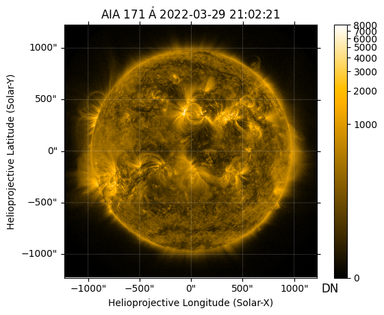

m_aia = correct_degradation(update_pointing(m_aia, pointing_table=pointing_table), correction_table=correction_table)

m_aia.peek(vmin=0, vmax=8000)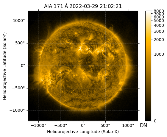

The SDO/AIA and STEREO-A/SECCHI/EUVI data are not been normalized for exposure time, whereas the Solar Orbiter/EUI/FSI data (level 2) are normalized for exposure time.

m_secchi.peek()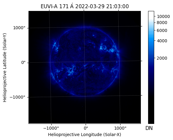

m_eui.peek()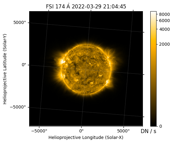

We normalize the SDO/AIA and STEREO-A/SECCHI/EUVI data for exposure time.

m_aia = m_aia / m_aia.exposure_time
m_secchi = m_secchi / m_secchi.exposure_time

m_aia.peek()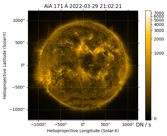

m_secchi.peek()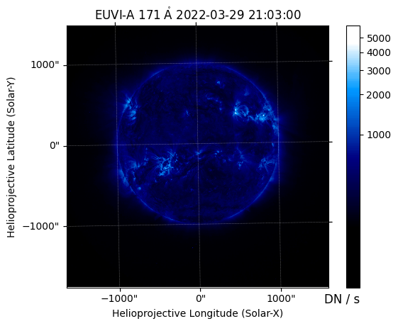

We can plot the position of the corrected center of the AR on the EUV maps.

fig = plt.figure(figsize=(15, 5))
for i, m in enumerate([m_aia, m_eui, m_secchi]):
    ax = fig.add_subplot(1, 3, i+1, projection=m)
    m.plot(axes=ax, clip_interval=(1, 99.99)*u.percent)
    ax.plot_coord(ar_center_corrected, marker='o', color='C3')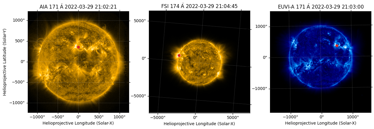

We can plot the region of interest on the EUV maps.

ar_width = 700*u.arcsec
ar_height = 700*u.arcsec

fig = plt.figure(figsize=(15, 5))
for i, m in enumerate([m_aia, m_eui, m_secchi]):
    ax = fig.add_subplot(1, 3, i+1, projection=m)
    m.plot(axes=ax, clip_interval=(1, 99.99)*u.percent)
    ar_center_corrected_transformed = ar_center_corrected.transform_to(m.coordinate_frame)
    blc = SkyCoord(Tx=ar_center_corrected_transformed.Tx-ar_width/2,
                   Ty=ar_center_corrected_transformed.Ty-ar_height/2,
                   frame=ar_center_corrected_transformed)
    m.draw_quadrangle(blc, width=ar_width, height=ar_height, edgecolor='C3', lw=1)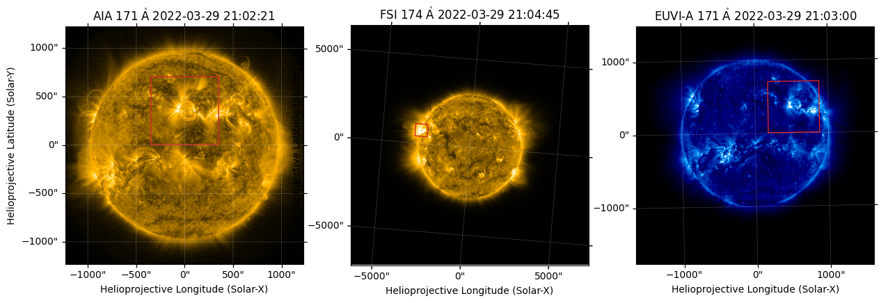

We can rotate the maps such that the y-axis of the images is aligned with the solar north using sunpy.map.Map.rotate.

fig = plt.figure(figsize=(15, 5))
for i, m in enumerate([m_aia, m_eui, m_secchi]):
    ax = fig.add_subplot(1, 3, i+1, projection=m)
    m_rot = m.rotate(missing=0.0)
    m_rot.plot(axes=ax, clip_interval=(1, 99.99)*u.percent)
    ar_center_corrected_transformed = ar_center_corrected.transform_to(m_rot.coordinate_frame)
    blc = SkyCoord(Tx=ar_center_corrected_transformed.Tx-ar_width/2,
                   Ty=ar_center_corrected_transformed.Ty-ar_height/2,
                   frame=ar_center_corrected_transformed)
    m_rot.draw_quadrangle(blc, width=ar_width, height=ar_height, edgecolor='C3', lw=1)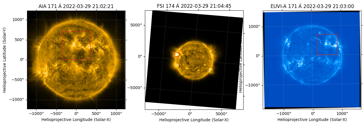

We can now crop each full disk image to the appropriate region.

m_cutouts = []
for m in [m_aia, m_eui, m_secchi]:
    ar_center_corrected_transformed = ar_center_corrected.transform_to(m.coordinate_frame)
    blc = SkyCoord(Tx=ar_center_corrected_transformed.Tx-ar_width/2,
                   Ty=ar_center_corrected_transformed.Ty-ar_height/2,
                   frame=ar_center_corrected_transformed)
    # Each map is rotated prior to submapping such that the selection is aligned with the coordinate grid
    m_rot = m.rotate(missing=0.0)
    m_cutout = m_rot.submap(blc, width=ar_width, height=ar_height)
    m_cutouts.append(m_cutout)

fig = plt.figure(figsize=(15, 5))
for i, m in enumerate(m_cutouts):
    ax = fig.add_subplot(1, 3, i+1, projection=m)
    m.plot(axes=ax, clip_interval=(1, 99.99)*u.percent)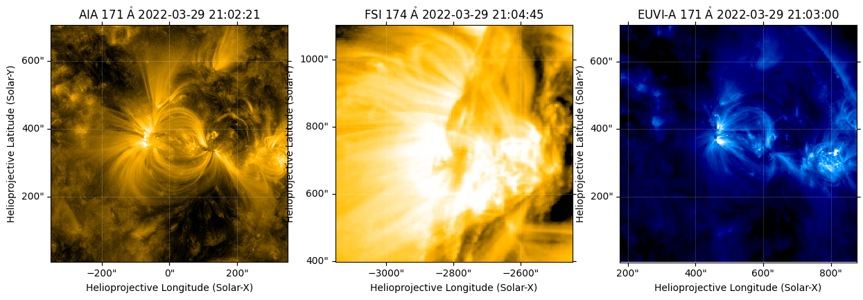

Calculate PFSS from HMI Synoptic Magnetogram

We can calculate a potential field source surface (PFSS) solution from the HMI synoptic magnetogram using sunkit-magex package.

We first resample the HMI synoptic map to speed up the calculation of our field extrapolation.

m_hmi.data.shape

(1440, 3600)

m_hmi_resample = m_hmi.resample((1080, 540)*u.pix)

m_hmi_resample.data.shape

(540, 1080)

from sunkit_magex import pfss

nr = 70    # number of cells in the radial direction
rss = 2.5  # radius of the source surface in R_sun
pfss_input = pfss.Input(m_hmi_resample, nr, rss)

pfss_output = pfss.pfss(pfss_input)

Let’s plot the radial component of the magnetic field at the source surface (2.5 Rs) and the polarity inversion lines (PILs).

fig = plt.figure()
ax = fig.add_subplot(111, projection=pfss_output.source_surface_br)
im = pfss_output.source_surface_br.plot(axes=ax)
ax.plot_coord(pfss_output.source_surface_pils[0], color='k')
fig.colorbar(im, ax=ax);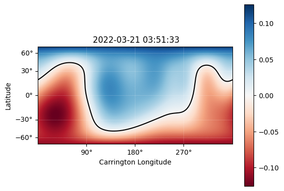

Trace Magnetic Field Lines

Let’s trace some field lines through the extrapolated field.

To do this, we need to choose a set of seed points from which to trace our field lines. We want to select only the seed points that are within a certain area around the active region. We need to make the following transformations because we want to express our boundaries in terms of the active region boundary as identified by our SDO/AIA cutout.

change_obstime_frame = lambda x,y: x.replicate_without_data(observer=x.observer.replicate(obstime=y), obstime=y)

new_frame = change_obstime_frame(m_hmi.coordinate_frame, m_cutouts[0].date)
new_frame

<HeliographicCarrington Frame (obstime=2022-03-29T21:02:21.350, rsun=695700.0 km, observer=<HeliographicStonyhurst Coordinate (obstime=2022-03-29T21:02:21.350, rsun=695700.0 km): (lon, lat, radius) in (deg, deg, m)
    (0., -7.02110576, 1.48994814e+11)>)>

blc_ar_synop = change_obstime(m_cutouts[0].bottom_left_coord.transform_to(new_frame),
                              m_hmi.date)
trc_ar_synop = change_obstime(m_cutouts[0].top_right_coord.transform_to(new_frame),
                              m_hmi.date)

We mask all those points that are above -10 G and fall outside of the bounding box defined above.

masked_pix_y, masked_pix_x = np.where(m_hmi_resample.data < -1e1)
seeds = m_hmi_resample.pixel_to_world(masked_pix_x*u.pix, masked_pix_y*u.pix).make_3d()
in_lon = np.logical_and(seeds.lon > blc_ar_synop.lon, seeds.lon < trc_ar_synop.lon)
in_lat = np.logical_and(seeds.lat > blc_ar_synop.lat, seeds.lat < trc_ar_synop.lat)
seeds = seeds[np.where(np.logical_and(in_lon, in_lat))]
seeds

<HeliographicCarrington Coordinate (obstime=2022-03-21T03:51:33.000, rsun=695700.0 km, observer=<HeliographicStonyhurst Coordinate (obstime=2022-03-21T03:51:33.000, rsun=695700.0 km): (lon, lat, radius) in (deg, deg, m)
    (0., -7.02110576, 1.48994814e+11)>): (lon, lat, radius) in (deg, deg, km)
    [(48.88333333, -5.63254256, 695700.),
     (69.55      , -5.63254256, 695700.),
     (74.88333333, -5.63254256, 695700.), ...,
     (62.55      , 41.38466759, 695700.),
     (63.88333333, 41.38466759, 695700.),
     (71.55      , 41.38466759, 695700.)]>

We can trace field lines from seeds specified above.

ds = 0.01
max_steps = int(np.ceil(10 * nr / ds))
tracer = pfss.tracing.PerformanceTracer(step_size=ds, max_steps=max_steps)
fieldlines = tracer.trace(SkyCoord(seeds), pfss_output)

We also want to adjust obstime of all coordinates to coincide with AR at disk center. By default, each field line will have the obstime of the map that the field extrapolation was computed from. Additionally, we will choose only the close field lines.

fieldlines.closed_field_lines[0].coords.observer

<HeliographicStonyhurst Coordinate (obstime=2022-03-21T03:51:33.000, rsun=695700.0 km): (lon, lat, radius) in (deg, deg, m)
    (0., -7.02110576, 1.48994814e+11)>

fline_coords = [change_obstime(f.coords, m_aia.date) for f in fieldlines.closed_field_lines if f.coords.shape[0]>500]

len(fline_coords)

fline_coords[0].observer

<HeliographicStonyhurst Coordinate (obstime=2022-03-29T21:02:21.350, rsun=695700.0 km): (lon, lat, radius) in (deg, deg, m)
    (0., -7.02110576, 1.48994814e+11)>

Finally, let’s plot these field lines on top of our EUV images.

fig = plt.figure(figsize=(18, 5))
for i, m in enumerate(m_cutouts):
    ax = fig.add_subplot(1, 3, i+1, projection=m)
    m.plot(axes=ax, title=f'{m.observatory} {m.detector} {m.wavelength.to_string(format="latex")}')
    bounds = ax.axis()
    for c in fline_coords[::5]:
        ax.plot_coord(c, lw=1, color='C2', alpha=0.75)
    ax.axis(bounds)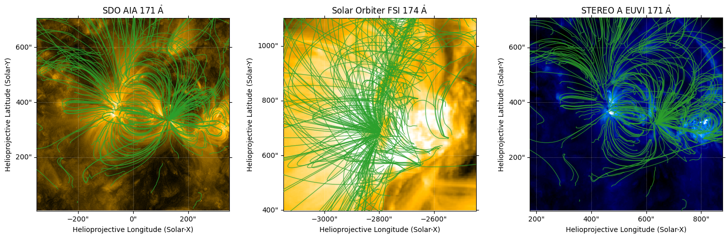

Figure 1 from the SunPy Paper (2023)

We can plot Figure 1 from the SunPy paper (2023).

from matplotlib.patches import ConnectionPatch
from matplotlib.gridspec import GridSpec

def add_connectors(ax1, ax2, p1, p2, color='k', lw=1):
    con1 = ConnectionPatch(
        (0, 1), ax1.wcs.world_to_pixel(p1), 'axes fraction', 'data', axesA=ax2, axesB=ax1,
        arrowstyle='-', color=color, lw=lw
    )
    con2 = ConnectionPatch(
        (1, 1), ax1.wcs.world_to_pixel(p2), 'axes fraction', 'data', axesA=ax2, axesB=ax1,
        arrowstyle='-', color=color, lw=lw
    )
    ax2.add_artist(con1)
    ax2.add_artist(con2)

h_w_ratio = 21 / 18
width = 12
frame_color = 'C3'
fig = plt.figure(figsize=(width, width*h_w_ratio))
gs = GridSpec(3, 3, figure=fig)
# Plot HMI synoptic map
ax = fig.add_subplot(gs[0, :2], projection=m_hmi)
m_hmi.plot(axes=ax, title='HMI Synoptic Magnetogram (CR 2255)')
m_hmi.draw_quadrangle(blc_ar_synop, top_right=trc_ar_synop, color=frame_color)
ax.coords[0].grid(color='k')
ax.coords[1].grid(color='k')
# Plot spacecraft locations
ax = fig.add_subplot(gs[0, 2], projection='polar')
ax.plot(0, 0, marker='o', markersize=15, label='Sun', color='yellow')
for m in m_cutouts:
    sat = m.observatory
    coord = m.observer_coordinate
    ax.plot(coord.lon.to('rad'), coord.radius.to(u.AU), 'o', label=sat)
    ax.text(coord.lon.to_value('rad')*1.15, coord.radius.to_value(u.AU)*0.95, sat)
ax.set_theta_zero_location('S')
ax.set_rlabel_position(225)
ax.set_rlim(0, 1.1)
# Plot full-disk EUV images
full_disk_axes = []
for i, m in enumerate([m_aia, m_eui, m_secchi]):
    ax = fig.add_subplot(gs[1, i], projection=m)
    m.plot(axes=ax, clip_interval=(1, 99.99)*u.percent, title=f'{m.observatory} {m.detector} {m.wavelength.to_string(format="latex")}')
    m.draw_quadrangle(m_cutouts[i].bottom_left_coord, top_right=m_cutouts[i].top_right_coord, color=frame_color, lw=1)
    if i:
        ax.coords[1].set_axislabel(' ')
    ax.coords[0].set_axislabel(' ')
    full_disk_axes.append(ax)
    ax.coords[1].set_ticklabel(rotation=90)
# Plot EUV cutouts with field lines
for i, m in enumerate(m_cutouts):
    ax = fig.add_subplot(gs[2, i], projection=m)
    m.plot(
        axes=ax,
        title=False,
        clip_interval=(1, 99.99)*u.percent,
    )
    bounds = ax.axis()
    for c in fline_coords[::8]:
        ax.plot_coord(c, lw=1, color='C2', alpha=0.75)
    ax.axis(bounds)
    if i:
        ax.coords[1].set_axislabel(' ')
    bottom_right = SkyCoord(Tx=m_cutouts[i].top_right_coord.Tx, Ty=m_cutouts[i].bottom_left_coord.Ty, frame=m_cutouts[i].coordinate_frame)
    add_connectors(full_disk_axes[i], ax, m_cutouts[i].bottom_left_coord, bottom_right, color=frame_color, lw=1)
    ax.grid(alpha=0)
    ax.coords[0].set_ticks(direction='in', color=frame_color)
    ax.coords[1].set_ticks(direction='in', color=frame_color)
    ax.coords[0].frame.set_color(frame_color)
    ax.coords[0].frame.set_linewidth(1)
    ax.coords[1].frame.set_color(frame_color)
    ax.coords[1].frame.set_linewidth(1)
    ax.coords[1].set_ticklabel(rotation=90)

plt.subplots_adjust(hspace=0.0)
plt.show()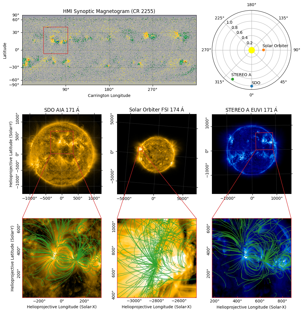

References

Barnes, W. T., Christe, S., Freij, N., et al. 2023, Frontiers in Astronomy and Space Sciences, 10, 1076726, https://arxiv.org/abs/2304.09794

Mumford, S., Freij, N., Christe, S., et al. 2020, The Journal of Open Source Software, 5, 1832

Stansby, D., Yeates, A., & Badman, S. 2020, The Journal of Open Source Software, 5, 2732

Sun, X. 2018, https://arxiv.org/abs/1801.04265

The SunPy Community, Barnes, W. T., Bobra, M. G., et al. 2020, The Astrophysical Journal, 890 (American Astronomical Society), 68, https://iopscience.iop.org/article/10.3847/1538-4357/ab4f7a

The SunPy Community, Mumford, S. J., Christe, S., et al. 2015, Computational Science and Discovery, 8, 014009, https://arxiv.org/abs/1505.02563