Calculating Derivatives of a 1D Scalar Function in Python

There are four techniques to compute derivatives: hand-coded analytical derivative, finite differentiation, symbolic differentiation, and automatic differentiation (Margossian 2019). In this post, I will demonstrate how to find the derivative of a simple 1D scalar function, f(x) = x^2 + \sin(3x), using each of these four methods in Python within the interval x \in [0, \pi].

1 Hand-coded analytical derivative

You can find the analytical derivative of the fucntion f(x) = x^2 + \sin(3x) using the table of derivatives learned in your Calculus course.

\begin{align*} \frac{d}{dx} f(x) & = \frac{d}{dx} (x^2 + \sin(3x)) \\ & = \frac{d}{dx} x^2 + \frac{d}{dx} \sin(3x) \\ & = 2x + 3\cos(3x) \end{align*}

Thus, for every x,

f'(x) = 2x + 3\cos(3x)

According to the previous post where I explained how to draw a 1D scalar function in Python, I will plot f(x) and its derivative f'(x) using Matplotlib.

Code

import matplotlib.pyplot as plt

plt.rcParams.update({
    "text.usetex": True,
    "font.family": "Helvetica",
    "font.size": 15,
    "figure.figsize": (8, 6)
})

import numpy as np
import matplotlib.pyplot as plt

func = lambda x: x**2 + np.sin(3*x)
d_func = lambda x: 2*x + 3*np.cos(3*x)

x = np.linspace(0, np.pi, 100)
f = func(x)
df_dx = d_func(x)

plt.plot(x, f, label=r"$f(x)$")
plt.plot(x, df_dx, label=r"$f'(x)$")
plt.axvline(0, color='k')
plt.axhline(0, color='k')
plt.xlabel(r"$x$")
plt.legend()
plt.show()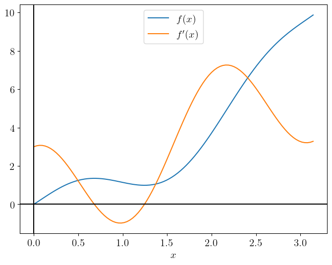

2 Finite differentiation

You can derive the following finite differentiation formulae using Taylor’s theorem.

2.1 Finite differentiation formulae

Forward difference
- 1st order accuracy f'(x) = \frac{f(x+h) - f(x)}{h} + \mathcal{O}(h)
- 2nd order accuracy f'(x) = \frac{-3f(x) + 4f(x+h) - f(x+2h)}{2h} + \mathcal{O}(h^2)
Backward difference
- 1st order accuracy f'(x) = \frac{f(x) - f(x-h)}{h} + \mathcal{O}(h)
- 2nd order accuracy f'(x) = \frac{3f(x) - 4f(x-h) + f(x-2h)}{2h} + \mathcal{O}(h^2)
Central difference
- 2nd order accuracy f'(x) = \frac{f(x+h) - f(x-h)}{2h} + \mathcal{O}(h^2)

2.2 Implementation using `NumPy`

NumPy arrays make the implementation of finite differentitation very straightforward. It’s important to note that at the left boundary (x=0), I use the forward difference, while at the right boundary (x=\pi), I use the backward difference. Within the domain (0<x<\pi), I use the central difference.

import numpy as np
import matplotlib.pyplot as plt

func = lambda x: x**2 + np.sin(3*x)

x = np.linspace(0, np.pi, 100)
f = func(x)

# calculate the spacing dx 
dx = x[1]-x[0]
# you can use np.diff
# dx = np.diff(x)[0] or
# dx = np.mean(np.diff(x))

# create an array with the same shape as `f`
df_dx = np.zeros_like(f)

# forward difference (1st order) at the left boundary
df_dx[0] = (f[1] - f[0]) / dx

# backward difference (1st order) at the right boundary
df_dx[-1] = (f[-1] - f[-2]) / dx

# central difference (2nd accuracy) within the domain
df_dx[1:-1] = (f[2:] - f[:-2]) / (2*dx)

# plot for comparison
exact_d_func = lambda x: 2*x + 3*np.cos(3*x)
df_dx_exact = exact_d_func(x)
plt.plot(x, df_dx_exact, 'b-', lw=3, label="exact")
plt.plot(x, df_dx, 'r--', lw=3, label="finite diff.")
plt.axvline(0, color='k')
plt.axhline(0, color='k')
plt.xlabel(r"$x$")
plt.ylabel(r"$f'(x)$")
RMSE = np.sqrt(np.mean((df_dx_exact - df_dx)**2))
plt.title(f"RMSE: {RMSE:.3e}")
plt.legend()
plt.show()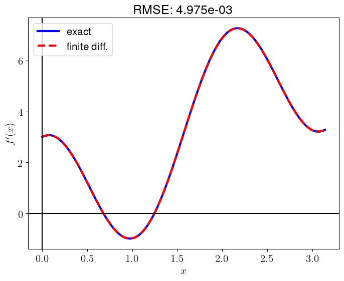

In the case of using 1st order accuracy formulae, the errors at the boundaries are

print('1st order')
print(f'dx   : {dx:.4f}')
print(f'left : {np.abs(df_dx[0] - df_dx_exact[0]):.4f}')
print(f'right: {np.abs(df_dx[-1] - df_dx_exact[-1]):.4f}')

1st order
dx   : 0.0317
left : 0.0272
right: 0.0272

If we use the 2nd order accuracy formulae at the boundaries instead, we get the following errors:

import numpy as np
import matplotlib.pyplot as plt

func = lambda x: x**2 + np.sin(3*x)

x = np.linspace(0, np.pi, 100)
f = func(x)

# calculate the spacing dx 
dx = x[1]-x[0]
# you can use np.diff
# dx = np.diff(x)[0] or
# dx = np.mean(np.diff(x))

# create an array with the same shape as `f`
df_dx = np.zeros_like(f)

# forward difference (2nd order) at the left boundary
df_dx[0] = (-3*f[0] + 4*f[1] - f[2]) / (2*dx)

# backward difference (2nd order) at the right boundary
df_dx[-1] = (3*f[-1] - 4*f[-2] + f[-3]) / (2*dx)

# central difference (2nd accuracy) within the domain
df_dx[1:-1] = (f[2:] - f[:-2]) / (2*dx)

# plot for comparison
exact_d_func = lambda x: 2*x + 3*np.cos(3*x)
df_dx_exact = exact_d_func(x)
plt.plot(x, df_dx_exact, 'b-', lw=3, label="exact")
plt.plot(x, df_dx, 'r--', lw=3, label="finite diff.")
plt.axvline(0, color='k')
plt.axhline(0, color='k')
plt.xlabel(r"$x$")
plt.ylabel(r"$f'(x)$")
RMSE = np.sqrt(np.mean((df_dx_exact - df_dx)**2))
plt.title(f"RMSE: {RMSE:.3e}")
plt.legend()
plt.show()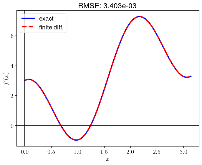

print('2nd order')
print(f'dx^2 : {dx**2:.4f}')
print(f'left : {np.abs(df_dx[0] - df_dx_exact[0]):.4f}')
print(f'right: {np.abs(df_dx[-1] - df_dx_exact[-1]):.4f}')

2nd order
dx^2 : 0.0010
left : 0.0090
right: 0.0090

np.allclose(df_dx_exact, df_dx)

False

np.allclose(df_dx_exact, df_dx, atol=1e-2)

True

2.2.1 `numpy.gradient`

There is a function for finite differentiation in NumPy.

import numpy as np
import matplotlib.pyplot as plt

func = lambda x: x**2 + np.sin(3*x)

x = np.linspace(0, np.pi, 100)
f = func(x)

# calculate the spacing dx 
dx = x[1]-x[0]

# calculate derivatives of `f` using np.gradient (2nd order)
df_dx_npgrad = np.gradient(f, dx, axis=0, edge_order=2)

# plot for comparison
exact_d_func = lambda x: 2*x + 3*np.cos(3*x)
df_dx_exact = exact_d_func(x)
plt.plot(x, df_dx_exact, 'b-', lw=3, label="exact")
plt.plot(x, df_dx_npgrad, 'r--', lw=3, label="finite diff. (np.gradient)")
plt.axvline(0, color='k')
plt.axhline(0, color='k')
plt.xlabel(r"$x$")
plt.ylabel(r"$f'(x)$")
RMSE = np.sqrt(np.mean((df_dx_exact - df_dx_npgrad)**2))
plt.title(f"RMSE: {RMSE:.3e}")
plt.legend()
plt.show()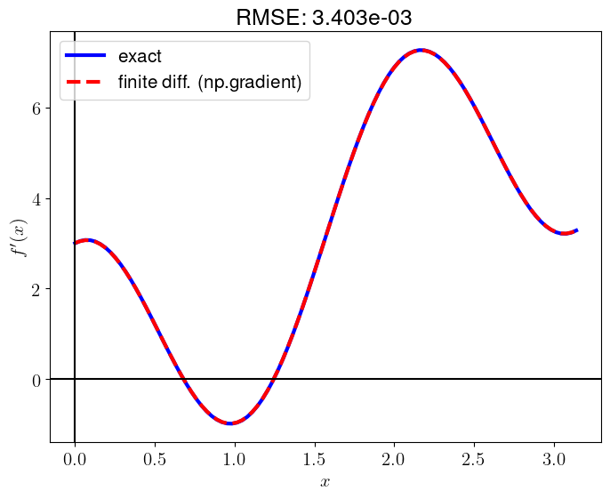

This computes the same value as manually computed.

np.allclose(df_dx, df_dx_npgrad)

True

2.3 Implementation using `findiff`

There is a convenient library for finite differentiation in Python: findiff

import numpy as np
import matplotlib.pyplot as plt
from findiff import FinDiff

func = lambda x: x**2 + np.sin(3*x)

x = np.linspace(0, np.pi, 100)
f = func(x)

# calculate the spacing dx 
dx = x[1]-x[0]

# construct the differential operator: FinDiff(axis, spacing, degree)
d_dx = FinDiff(0, dx, 1) 

df_dx_findiff = d_dx(f)

# plot for comparison
exact_d_func = lambda x: 2*x + 3*np.cos(3*x)
df_dx_exact = exact_d_func(x)
plt.plot(x, df_dx_exact, 'b-', lw=3, label="exact")
plt.plot(x, df_dx_findiff, 'r--', lw=3, label="finite diff. (findiff)")
plt.axvline(0, color='k')
plt.axhline(0, color='k')
plt.xlabel(r"$x$")
plt.ylabel(r"$f'(x)$")
RMSE = np.sqrt(np.mean((df_dx_exact - df_dx_findiff)**2))
plt.title(f"RMSE: {RMSE:.3e}")
plt.legend()
plt.show()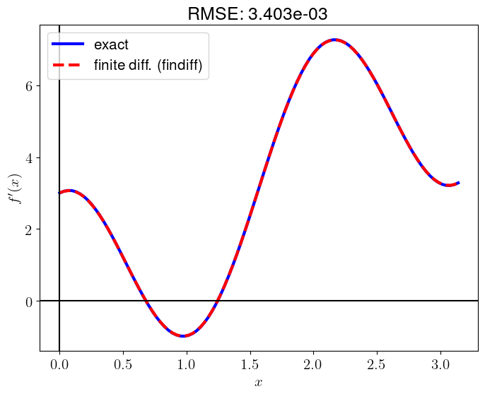

By default, findiff uses 2nd order accuray.

np.allclose(df_dx, df_dx_findiff)

True

You can also find finite difference coefficients using this library. (see Section 2.1)

import findiff
# coefficients of 2nd order accuracy formulae for 1st derivative
findiff.coefficients(deriv=1, acc=2)

{'center': {'coefficients': array([-0.5,  0. ,  0.5]),
  'offsets': array([-1,  0,  1]),
  'accuracy': 2},
 'forward': {'coefficients': array([-1.5,  2. , -0.5]),
  'offsets': array([0, 1, 2]),
  'accuracy': 2},
 'backward': {'coefficients': array([ 0.5, -2. ,  1.5]),
  'offsets': array([-2, -1,  0]),
  'accuracy': 2}}

np.allclose(df_dx_exact, df_dx_findiff)

False

np.allclose(df_dx_exact, df_dx_findiff, atol=1e-2)

True

2.4 Implementation using `numdifftools`

There is another convenient library for automatic numerical differentiation in Python: numdifftools

import numpy as np
import matplotlib.pyplot as plt
import numdifftools as nd

func = lambda x: x**2 + np.sin(3*x)

# construct a derivative function (FD)
d_func = nd.Derivative(func, n=1)

x = np.linspace(0, np.pi, 100)
df_dx_numdifftools = d_func(x)

# plot for comparison
exact_d_func = lambda x: 2*x + 3*np.cos(3*x)
df_dx_exact = exact_d_func(x)
plt.plot(x, df_dx_exact, 'b-', lw=3, label="exact")
plt.plot(x, df_dx_numdifftools, 'r--', lw=3, label="finite diff. (numdifftools)")
plt.axvline(0, color='k')
plt.axhline(0, color='k')
plt.xlabel(r"$x$")
plt.ylabel(r"$f'(x)$")
RMSE = np.sqrt(np.mean((df_dx_exact - df_dx_numdifftools)**2))
plt.title(f"RMSE: {RMSE:.3e}")
plt.legend()
plt.show()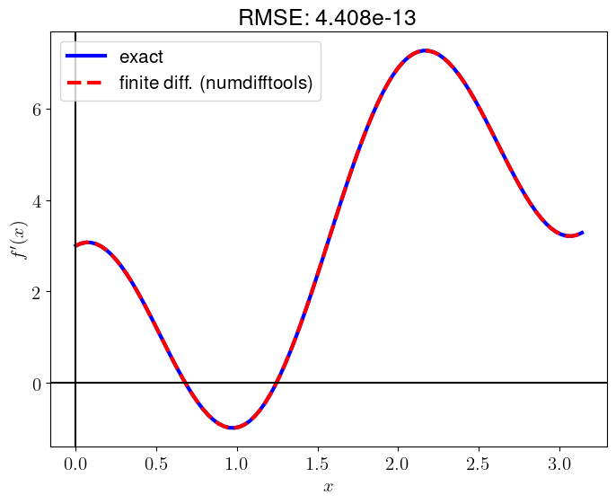

Since this library uses an adaptive finite differences with a Richardson extrapolation methodology, the result is maximally accurate.

np.allclose(df_dx_exact, df_dx_numdifftools)

True

3 Symbolic differentiation

3.1 Implementation using `Sympy`

By using SymPy, we can symbolically differentiate f(x) = x^2 + \sin(3x)

from sympy import symbols, sin, diff
x = symbols('x')
f = x**2 + sin(3*x)
f

\displaystyle x^{2} + \sin{\left(3 x \right)}

df_dx_sympy = diff(f, x)
df_dx_sympy

\displaystyle 2 x + 3 \cos{\left(3 x \right)}

As I mentioned in the previous post, SymPy also supports plotting of a function.

from sympy.plotting import plot
p1 = plot(f, (x, 0, np.pi), legend=True, show=False, label="$f(x)$", ylabel='')
p2 = plot(df_dx_sympy, (x, 0, np.pi), legend=True, show=False, label=r"$f'(x)$", ylabel='')
p1.extend(p2)
p1.show()

4 Automatic differentiation

In mathematics and computer algebra, automatic differentiation (auto-differentiation, autodiff, or AD), also called algorithmic differentiation, computational differentiation, is a set of techniques to evaluate the partial derivative of a function specified by a computer program. #

The efficient implementation of automatic differentiation is quite challenging. However, since the backpropagation is used to minimize loss in neural networks and is essentially a reverse-mode automatic differentiation, most deep learning libraries natively support automatic differentiation tools. In this post, I will demonstrate how to use automatic differentiation in Python with TensorFlow, PyTorch, and JAX.

4.1 Implementation using `TensorFlow`

TensorFlow is an end-to-end open source platform for machine learning.

import numpy as np
import matplotlib.pyplot as plt
import tensorflow as tf

func = lambda x: x**2 + tf.math.sin(3*x)

x = tf.linspace(0.0, tf.constant(np.pi), 100)

# calculate derivatives of `f`
with tf.GradientTape() as tape:
    tape.watch(x)
    f = func(x)
    df_dx_tf = tape.gradient(f, x)

df_dx_tf = df_dx_tf.numpy()

# plot for comparison
exact_d_func = lambda x: 2*x + 3*np.cos(3*x)
x_numpy = x.numpy()
df_dx_exact = exact_d_func(x_numpy)
plt.plot(x_numpy, df_dx_exact, 'b-', lw=3, label="exact")
plt.plot(x_numpy, df_dx_tf, 'r--', lw=3, label="auto diff. (TensorFlow)")
plt.axvline(0, color='k')
plt.axhline(0, color='k')
plt.xlabel(r"$x$")
plt.ylabel(r"$f'(x)$")
RMSE = np.sqrt(np.mean((df_dx_exact - df_dx_tf)**2))
plt.title(f"RMSE: {RMSE:.3e}")
plt.legend()
plt.show();

np.allclose(df_dx_exact, df_dx_tf)

True

4.2 Implementation using `PyTorch`

PyTorch is a Python package that supports tensors and dynamic neural networks in Python with strong GPU acceleration.

import numpy as np
import matplotlib.pyplot as plt
import torch

func = lambda x: x**2 + torch.sin(3*x)

x = torch.linspace(0, np.pi, 100)

# calculate derivatives of `f`
x.requires_grad = True
f = func(x)
df_dx_torch = torch.autograd.grad(f, x, grad_outputs=torch.ones_like(f), 
                            retain_graph=True, create_graph=True, allow_unused=True)[0]

df_dx_torch = df_dx_torch.detach().numpy()

# plot for comparison
exact_d_func = lambda x: 2*x + 3*np.cos(3*x)
x_numpy = x.detach().numpy()
df_dx_exact = exact_d_func(x_numpy)
plt.plot(x_numpy, df_dx_exact, 'b-', lw=3, label="exact")
plt.plot(x_numpy, df_dx_torch, 'r--', lw=3, label="auto diff. (PyTorch)")
plt.axvline(0, color='k')
plt.axhline(0, color='k')
plt.xlabel(r"$x$")
plt.ylabel(r"$f'(x)$")
RMSE = np.sqrt(np.mean((df_dx_exact - df_dx_torch)**2))
plt.title(f"RMSE: {RMSE:.3e}")
plt.legend()
plt.show()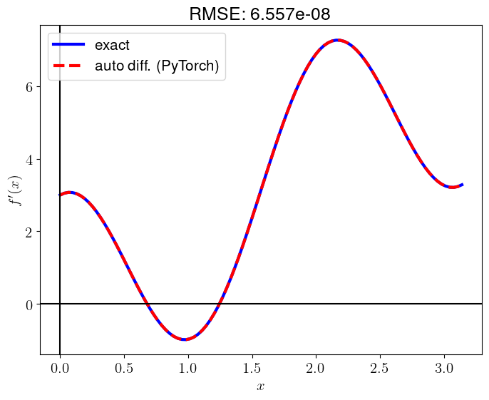

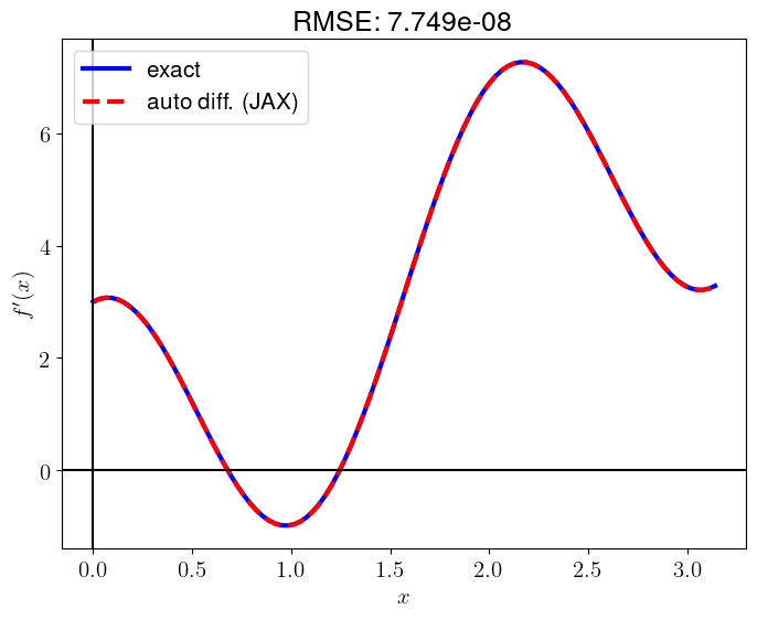
np.allclose(df_dx_exact, df_dx_torch)

True

4.3 Implementation using `JAX`

JAX is Autograd and XLA, brought together for high-performance numerical computing, including large-scale machine learning research.

import numpy as np
import matplotlib.pyplot as plt
import jax.numpy as jnp
import jax

func = lambda x: x**2 + jnp.sin(3*x)

x = jnp.linspace(0, jnp.pi, 100)

# calculate derivatives of `f`
df_dx_jax = jax.vmap(jax.grad(func))(x)

df_dx_jax = np.array(df_dx_jax)

# plot for comparison
exact_d_func = lambda x: 2*x + 3*np.cos(3*x)
x_numpy = np.array(x)
df_dx_exact = exact_d_func(x_numpy)
plt.plot(x_numpy, df_dx_exact, 'b-', lw=3, label="exact")
plt.plot(x_numpy, df_dx_jax, 'r--', lw=3, label="auto diff. (JAX)")
plt.axvline(0, color='k')
plt.axhline(0, color='k')
plt.xlabel(r"$x$")
plt.ylabel(r"$f'(x)$")
RMSE = np.sqrt(np.mean((df_dx_exact - df_dx_jax)**2))
plt.title(f"RMSE: {RMSE:.3e}")
plt.legend()
plt.show()

np.allclose(df_dx_exact, df_dx_jax)

True

References

Margossian, Charles C. 2019. “A Review of Automatic Differentiation and Its Efficient Implementation.” WIREs Data Mining and Knowledge Discovery 9 (4). https://doi.org/10.1002/WIDM.1305.

1 Hand-coded analytical derivative

2 Finite differentiation

2.1 Finite differentiation formulae

2.2 Implementation using NumPy

2.2.1 numpy.gradient

2.3 Implementation using findiff

2.4 Implementation using numdifftools